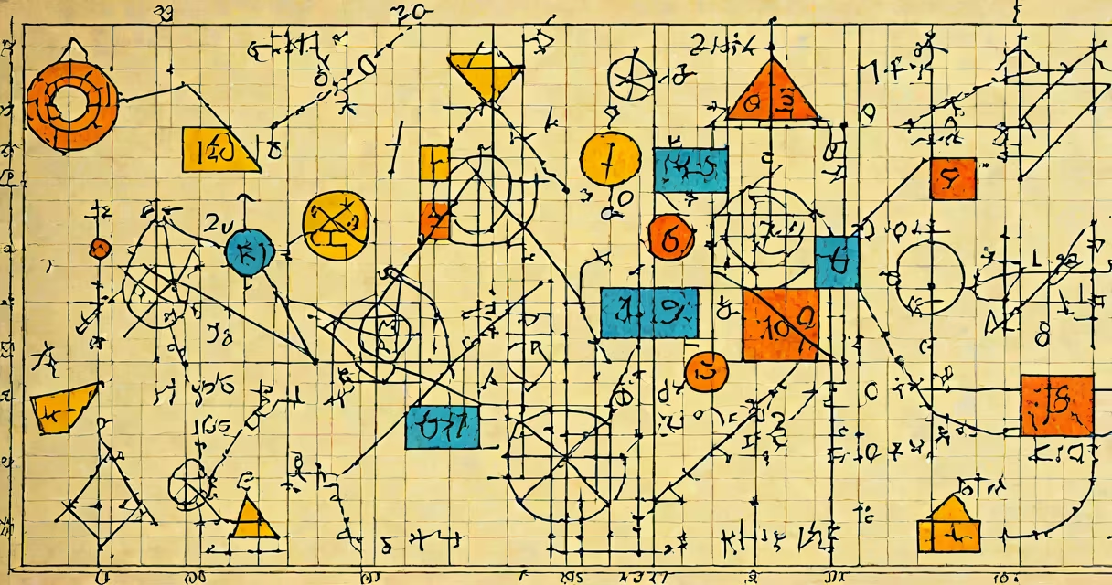
A complex math equation is a symbolic statement using numbers, variables, operations, and functions that expresses a relationship requiring multiple steps or advanced techniques to resolve. It often involves higher-order functions, multiple variables, or non-linear structures beyond basic arithmetic.
These equations define relationships between quantities that change in non-trivial ways. They appear in physics, engineering, economics, and computer science to model systems where outcomes depend on several interdependent factors. Solving them typically requires methods like integration, differentiation, matrix algebra, or numerical approximation.
For example, the Navier-Stokes equations-used to describe fluid flow-form a system of partial differential equations. These equations contain derivatives of velocity and pressure across space and time, making them impossible to solve exactly in most real-world cases. Instead, scientists use computational models to approximate solutions.
At their core, complex math equations follow the same logic as simpler ones: they state that two expressions are equal under certain conditions. But they introduce layers of abstraction through operators like summation (∑), integration (∫), or partial derivatives (∂/∂t).
Each symbol adds meaning. The integral sign ∫ denotes accumulation over a continuous domain. For instance, ∫₀¹ x² dx calculates the area under the curve y = x² from x = 0 to x = 1. This yields 1/3-a result derived via the Fundamental Theorem of Calculus.
When equations involve multiple variables and dependencies, solving becomes iterative. Consider the heat equation: ∂u/∂t = α∇²u. This describes how temperature u changes over time t due to spatial diffusion, governed by thermal diffusivity α. Solving it requires boundary conditions and finite difference methods in practice.
Complex math equations fall into categories based on structure and solution method. The table below outlines common types, their defining features, and real-world applications.
| Type | Key Features | Example | Use Case |
|---|---|---|---|
| Partial Differential Equation (PDE) | Multiple independent variables, derivatives in more than one direction | ∂²ψ/∂x² + ∂²ψ/∂y² = 0 (Laplace's equation) | Electrostatics, fluid dynamics |
| Nonlinear Algebraic System | Variables raised to powers >1, cross-term interactions | x³ + 2xy − y² = 5 | Robot kinematics, economic equilibrium models |
| Integral Equation | Unknown function appears inside an integral | f(x) = λ∫K(x,t)f(t)dt | Quantum mechanics, signal processing |
| Stochastic Differential Equation (SDE) | Includes random processes (e.g., Brownian motion) | dX_t = μX_t dt + σX_t dW_t | Financial modeling, population dynamics |
Some equations combine multiple types. The Schrödinger equation in quantum mechanics, for example, is a linear PDE involving both time and spatial derivatives, with complex-valued wavefunctions.
Complex math equations model phenomena that cannot be captured by simple addition or multiplication. In aerospace engineering, the Euler equations govern compressible fluid flow around aircraft wings. Engineers use these to predict lift and drag forces during design phases.
In finance, the Black-Scholes equation determines option prices based on volatility, time to expiration, and interest rates. It uses stochastic calculus and assumes market efficiency-conditions that don't always hold, but still provide a benchmark for pricing.
One non-obvious fact: many complex equations lack closed-form solutions. The three-body problem in celestial mechanics-predicting the motion of three masses under mutual gravity-has no general analytical solution. Scientists rely on simulations and perturbation theory instead.
People often assume that a complex math equation must have a unique solution. That's false. Some equations have infinite solutions, others none. For example, the equation sin(x) = 2 has no real solution because sine values are bounded between -1 and 1.
Another misconception is that complexity equals accuracy. A highly complex equation may fit data well but fail to generalize. Overfitting occurs when a model captures noise rather than underlying patterns. Cross-validation and regularization techniques help avoid this.
I once tested a neural network trained on climate data using a custom loss function based on a partial differential equation. The model performed well on training data but failed to predict droughts in new regions. The equation was mathematically sound but lacked physical constraints relevant to arid zones.
Simple equations like 2x + 3 = 7 involve one variable and basic operations. Their solution is a single number. Complex equations often return sets of solutions, functions, or numerical approximations.
Consider the quadratic equation ax² + bx + c = 0. Its solution is x = [-b ± √(b²−4ac)] / 2a-a formula derived through completing the square. While this is algebraically complex, it remains solvable in closed form.
Now compare it to the Lorenz system: dx/dt = σ(y−x), dy/dt = x(ρ−z)−y, dz/dt = xy−βz. This set of three coupled nonlinear ODEs exhibits chaotic behavior. Small changes in initial conditions lead to vastly different outcomes-known as the butterfly effect. There is no closed-form solution; only numerical simulation reveals trajectories.